
Neural Style Transfer (NST) takes the semantic structure of one image (the content) and renders it in the texture and visual style of another. It is based on the pre-trained VGG-19 Convolutional Neural Network (CNN). This implementation is inspired by the official TensorFlow tutorial Style Transfer, and extends it with stronger diagnostics (effective learning rate, optional Lipschitz constant estimation), reproducibility (logging, checkpoints), and clear notation.
A Quick Example
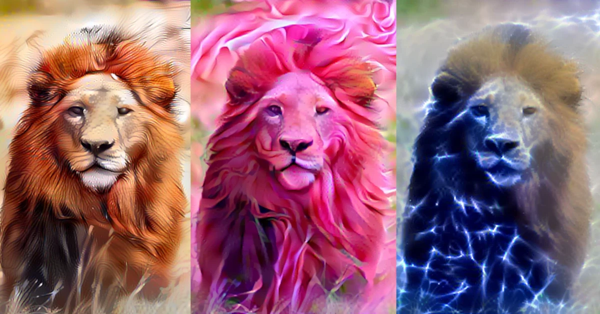
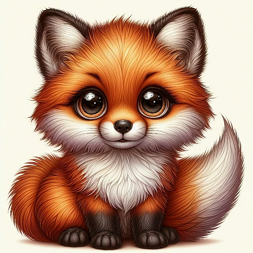
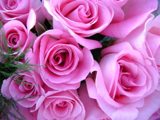
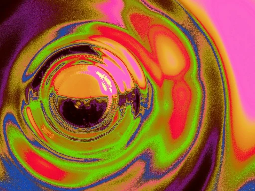
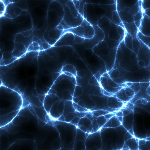
To illustrate the potential of NST, let Fig. 1 be the content image that we want to redraw using Fig. 2 as the style image. The result is the image in Fig. 3.
|
|
|
Fig. 1. The content image to be redrawn. |
Fig. 2. The style image used to redraw the content image in Fig. 1. |
Fig. 3. Neural Style Transfer: the content image (Fig. 1) is redrawn using the style image (Fig. 2). |
In particular, the lion’s fur texture has been replaced with the cartoon fox’s. In the top right corner of Fig. 3, we can see some smoothing issues (dark patches) as well as on the top of the lion’s head. This shows the model sensitivity to the parameters (you can tune them with command-line arguments and make your own tests). Nevertheless, the purpose of this project is to experiment with CNNs and see their potential for Generative AI.
Getting the code
You can download the code from its GitHub repository with
$ git clone https://github.com/CoffeeDynamics/Neural-Style-Transfer.gitThe sections below give some insights about the theory and the implementation, and show some example results.
Problem setup and notation
We optimise directly over the pixels of an image. Let $x$ be the optimisation variable (stylized image), $x_c$, the content image, and $x_s$, the style image. One has
\begin{equation}
x \in [0,1]^{H \times W \times 3},
\end{equation}
where $H$ and $W$ are the image height and width, and the final dimension of size 3 corresponds to RGB (Red – Green – Blue) colour channels.
A frozen VGG-19 provides perceptual features. For a layer $\ell$, the activation tensor is
\begin{equation}
\phi_\ell(x) \in \mathbb{R}^{H_\ell \times W_\ell \times C_\ell},
\end{equation}
where $H_\ell$ and $W_\ell$ are the spatial dimensions at layer $\ell$ and $C_\ell$ is the number of channels (filters).
We define the set of content layers,
\begin{equation}
L_c = \left\{\text{block5_conv2}\right\},
\end{equation}
and the set of style layers,
\begin{equation}
L_s = \left\{\text{block1_conv1}, \text{block2_conv1}, \text{block3_conv1},\\ \text{block4_conv1}, \text{block5_conv1}\right\}.
\end{equation}
To build style statistics, we flatten spatial dimensions so rows enumerate spatial locations and columns enumerate channels:
\begin{equation}
F_\ell(x) \in \mathbb{R}^{(H_\ell W_\ell)\times C_\ell}, \qquad
F_\ell(x)_{p,c} := \phi_\ell(x)_{i_p,j_p,c}.
\end{equation}
Here, $p$ indexes spatial positions after flattening, $(i_p,j_p)$ are the corresponding 2D coordinates, and $c$ indexes channels.
The normalized Gram matrix captures channel–channel correlations:
\begin{equation}
G_\ell(x) := \frac{1}{H_\ell W_\ell}F_\ell(x)^\top F_\ell(x) \in \mathbb{R}^{C_\ell \times C_\ell}.
\end{equation}
Loss terms
Content loss. Squared Euclidean distance of deep features:
\begin{equation}
L_{\mathrm{content}}(x,x_c) = \frac{1}{|L_c|}\sum_{\ell \in L_c} \left|\phi_\ell(x) – \phi_\ell(x_c)\right|_F^2.
\end{equation}
Here, $|\cdot|_F$ denotes the Frobenius norm, i.e., the Euclidean norm of all entries in the tensor after flattening.
Style loss. Squared Frobenius distance between Gram matrices across style layers:
\begin{equation}
L_{\mathrm{style}}(x,x_s) = \frac{1}{|L_s|}\sum_{\ell \in L_s} \left|G_\ell(x) – G_\ell(x_s)\right|_F^2.
\end{equation}
Total variation (TV) loss. Spatial regularizer that discourages high-frequency artefacts. The implementation uses TensorFlow’s isotropic form:
\begin{equation}
L_{\mathrm{TV}}(x) = \sum_{i,j} \sqrt{ \big(x_{i+1,j} – x_{i,j}\big)^2 + \big(x_{i,j+1} – x_{i,j}\big)^2 }.
\end{equation}
Here $i,j$ index spatial coordinates, and the sum is applied channel-wise across the three RGB channels.
Total objective. Weights $\alpha$ (content), $\beta$ (style), $\tau$ (TV) trade off structure, texture, and smoothness:
\begin{equation}
L(x) = \alpha L_{\mathrm{content}}(x,x_c) + \beta L_{\mathrm{style}}(x,x_s) + \tau L_{\mathrm{TV}}(x).
\end{equation}
This is the function minimized by our model.
VGG-19: why and how it’s used
VGG-19 is a deep CNN yet uniform: stacks of $3\times 3$ convolutions with max-pooling between blocks. Early layers encode colours and fine textures; mid layers encode motifs; deep layers encode semantics.
In NST:
- Content comes from a deep semantic layer:
block5_conv2. - Style comes from the first convolution layer of each block:
block{1..5}_conv1.
We keep the ImageNet-pre-trained weights frozen, turning VGG-19 into a stable perceptual feature extractor.
For a generic input of size $H\times W$ (resized so that $\max(H,W)\le 512$), Table 1 shows the shape evolution as information is propagated into the network.
| Block | Layer(s) | Output shape $(H_\ell \times W_\ell \times C_\ell)$ |
|---|---|---|
| — | Input | $H \times W \times 3$ |
| B1 | block1_conv1, block1_conv2 | $H \times W \times 64$ |
| MaxPooling | $\tfrac{H}{2}\times \tfrac{W}{2}\times 64$ | |
| B2 | block2_conv1, block2_conv2 | $\tfrac{H}{2}\times \tfrac{W}{2}\times 128$ |
| MaxPooling | $\tfrac{H}{4}\times \tfrac{W}{4}\times 128$ | |
| B3 | block3_conv1, block3_conv2, block3_conv3, block3_conv4 | $\tfrac{H}{4}\times \tfrac{W}{4}\times 256$ |
| MaxPooling | $\tfrac{H}{8}\times \tfrac{W}{8}\times 256$ | |
| B4 | block4_conv1, block4_conv2, block4_conv3, block4_conv4 | $\tfrac{H}{8}\times \tfrac{W}{8}\times 512$ |
| MaxPooling | $\tfrac{H}{16}\times \tfrac{W}{16}\times 512$ | |
| B5 | block5_conv1, block5_conv2, block5_conv3, block5_conv4 | $\tfrac{H}{16}\times \tfrac{W}{16}\times 512$ |
| MaxPooling | $\tfrac{H}{32}\times \tfrac{W}{32}\times 512$ |
Preprocessing
Both content and style images are automatically resized so their longest side is 512 pixels (aspect ratio preserved). They are converted to float32 tensors in $[0,1]$, and a batch dimension is added so the actual network input dimension is $1 \times H \times W \times 3$.
Optimisation and diagnostics
We optimise the pixels of $x$ (initialised from $x_c$) with the Adam optimiser and clip back to $[0,1]$ after each step.
To make optimiser behaviour observable, we log the effective learning rate:
\begin{equation}
\alpha_{\mathrm{eff}} = \frac{\alpha}{\sqrt{\hat v} + \epsilon},
\end{equation}
where $\alpha$ is the Adam base learning rate, $\hat v$ is the bias-corrected second-moment estimate, and $\epsilon$ is a small constant for numerical stability. We report min/mean/max of $\alpha_{\mathrm{eff}}$ across all pixels each iteration.
Optional Lipschitz estimation. With --optim, we estimate the largest eigenvalue, $L$, of the pixel-space Hessian via power iteration on Hessian–vector products, providing a stability heuristic. For vanilla gradient descent, the step size, $\eta$, must satisfy
\begin{equation}
\eta < \frac{2}{L}.
\end{equation}
Here $\eta$ denotes the learning rate of plain gradient descent (analogous to $\alpha$ in Adam). Although Adam is not plain GD, monitoring $\alpha_{\mathrm{eff}}\cdot L$ is informative: large values correlate with oscillations; tiny values with stagnation.
Command-line interface
The script is designed as a CLI. Minimal usage:
$ python neural_style_transfer.py --content path/to/content.jpg \
--style path/to/style.jpg --output out/stylized.pngKey flags:
--nsteps: number of steps (default: 1,000)--content_weight: content loss weight, $\alpha$ (default: 10,000)--style_weight: style loss weight, $\beta$ (default: 0.01)--tv_weight: total variation loss weight, $\tau$ (default: 300)- Adam hyperparameters:
--adam_learning_rate: learning rate (default: 0.01)--adam_beta_1: $\beta_1$ coefficient (default: 0.9)--adam_beta_2: $\beta_2$ coefficient (default: 0.999)--adam_epsilon: $\epsilon$ coefficient (default: 10-7)
- Logging and saving cadence:
--save_every: save every $N$ iterations (default: 100)--log_every: log every $N$ iterations (default: 1)--ckpt_write_every: write a checkpoint every $N$ iterations (default: 100)
- Checkpoints:
--resume: resume from checkpoint if available (default: start fresh)--resume_from: path to a specific checkpoint to restore (overrides--resume)--ckpt_in: path to checkpoint folder to restore from (default: None)--ckpt_keep_max: keep only the $N$ latest checkpoints (default: 5)
To see all flags:
$ python neural_style_transfer.py -hWhat gets saved
- Images: the style image, the initial content snapshot, periodic stylized results every
--save_everysteps, and a final image with suffix_final.png. Filenames embed the content/style base names and step count. - Checkpoints: TensorFlow checkpoints in
.../checkpoints/, storing both the image variable and optimiser state; can resume training exactly. - Logs: a
.txtlog with environment info and hyperparameters in the header. Each row reports: step, content/style/TV losses, total loss, and min/mean/max effective learning rates (plus $\alpha_{\mathrm{eff,max}}\cdot L$ if--optimis set).
Sample log excerpt (--optim not set):
#     Step        Content Loss          Style loss     Total Variation          Total Loss       alpha_eff_min      alpha_eff_mean       alpha_eff_max
         1      0.00000000e+00      7.93783552e+08      2.47124060e+07      8.18495936e+08      1.88675564e-08      2.50102585e-06      9.89065990e-02
         2      3.57562225e+06      6.26893376e+08      2.52307880e+07      6.55699776e+08      2.10574669e-08      5.46445506e-07      4.36682312e-04
3 7.84002150e+06 4.79356608e+08 2.58209200e+07 5.13017568e+08 2.55993946e-08 4.54668054e-07 4.92347754e-05Visualizing logs with gnuplot
The training script writes a structured .txt log. To make these diagnostics interpretable, I use a companion gnuplot.plt script to plot the content, style, TV, and total losses over steps, as shown in Fig. 4.
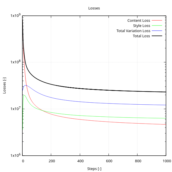
These plots complement the image snapshots: they show not just what the algorithm produces, but how it behaves during optimisation.
Results
The lion-fox illustration in Figs. 1-3 shows the core idea on a single pair. To examine the behaviour systematically, I generated 25 outputs by combining 5 content images (c1, …, c5) with 5 style images (s1, …, s5) using the default parameters (1,000 steps, $\alpha=10^4$, $\beta=10^{-2}$, and $\tau=3\cdot 10^2$), as shown in Table 2 (click on each image to enlarge it in another tab).
| Style s1 | Style s2 | Style s3 | Style s4 | Style s5 | |
|---|---|---|---|---|---|
 |  |  |  |  | |
Content c1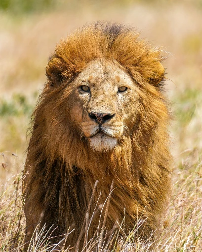 | 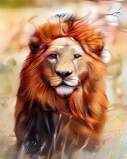 | 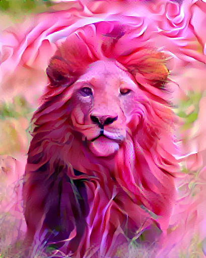 | 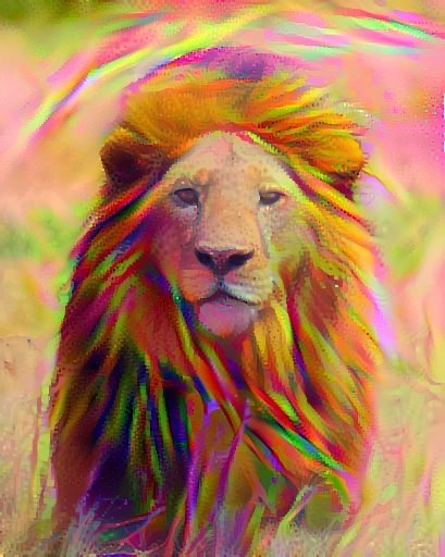 |  | 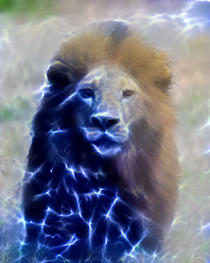 |
Content c2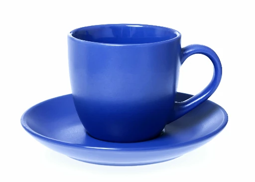 | 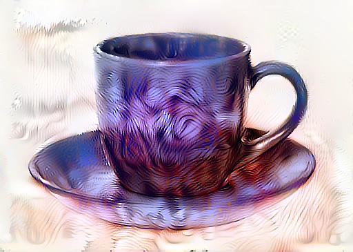 | 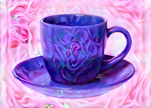 | 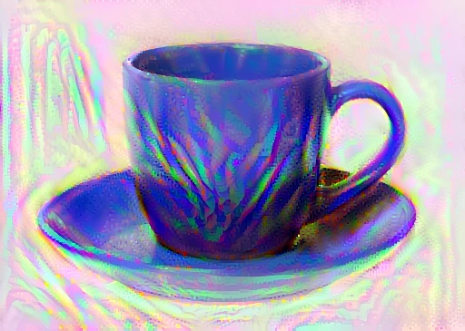 | 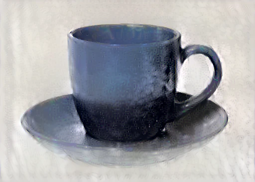 | 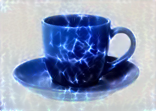 |
Content c3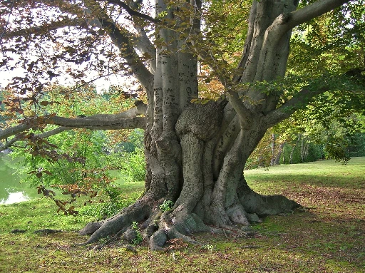 | 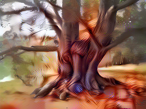 | 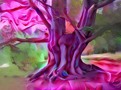 | 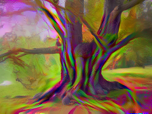 |  | 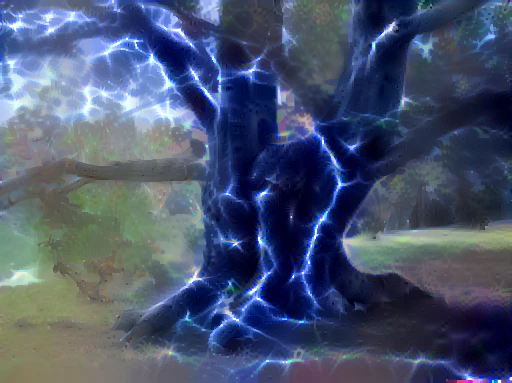 |
Content c4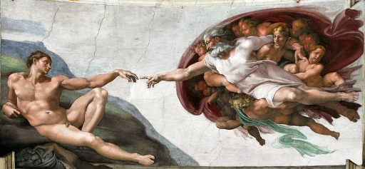 | 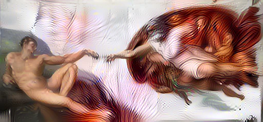 |  | 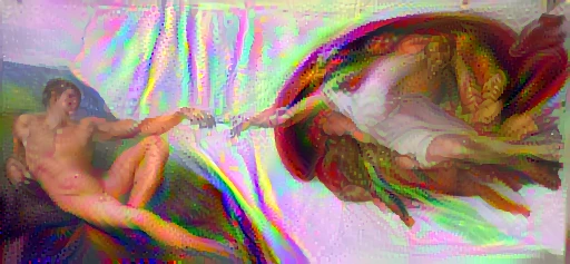 | 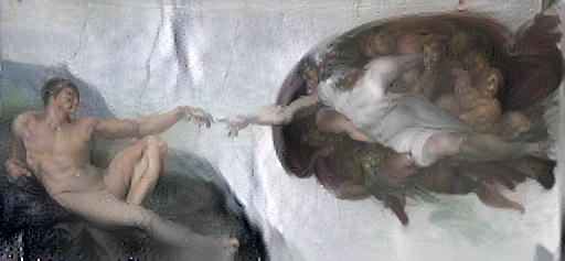 | 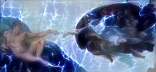 |
Content c5 | 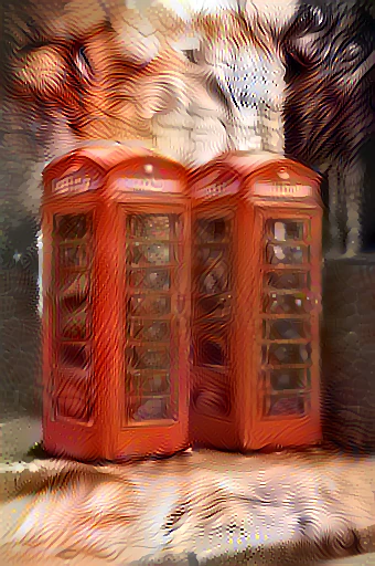 | 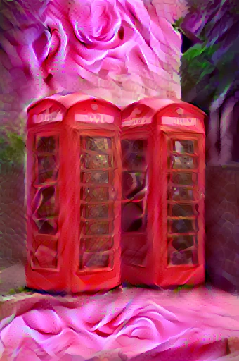 | 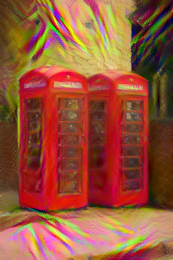 |  | 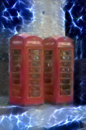 |
For example, the resulting image corresponding to the combination of content c1 and style s1 has been generated with
$ python neural_style_transfer.py --content content_files/c1.png \
   --style style_files/s1.png \
--output output_files/c1_s1/run0/result.pngAnd the final output image was written in output_files/c1_s1/run0/result_c1_s1_final.png in approximately 18 minutes on my desktop. These information are available in the log file result_c1_s1_log.txt written in the same folder.
Qualitative trends. Early iterations preserve structure with faint textures; mid-iterations intensify textures (TV regularisation curbs noise); at convergence, the balance is set by $(\alpha,\beta,\tau)$.
Conclusion
- VGG-19 as a perceptual extractor: deep content, shallow-to-mid style.
- Well-posed objective: content/style/TV terms with clear roles and weights.
- Pixel-space optimisation with visibility: effective learning rate logging, optional Lipschitz constant estimation, and gnuplot visualizations help explain stability and convergence.
- Reproducibility: deterministic preprocessing, logs, checkpoints, and periodic snapshots.
NST is both an artistic tool and a compact demonstration of deep learning’s flexibility: pre-trained CNN features, differentiable objectives, and iterative optimisation working together to transform images in a controlled, repeatable way.
Leave a Reply
You must be logged in to post a comment.